Survey Notes (EN)

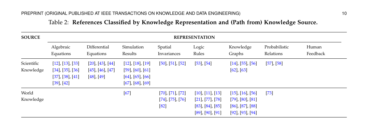
Citation

• Paper: Informed Machine Learning: A Taxonomy and Survey of Integrating Prior Knowledge into Learning Systems
• File: taxonomy_survey_2021_tkde.pdf

Core Purpose of This Survey

This paper does not propose one specific new informed ML method. Instead, it does three things:

1. It clarifies the conceptual boundary of informed machine learning.
2. It proposes a unified taxonomy describing where knowledge comes from, how it is represented, and how it enters a learning system.
3. It organizes existing methods according to that taxonomy, and points out the challenges and future directions associated with each path.

Therefore, the most important thing when reading this survey is not to memorize model names, but to first grasp its analytical framework.

Figure 1 Close Reading: Information Flow in Informed Machine Learning

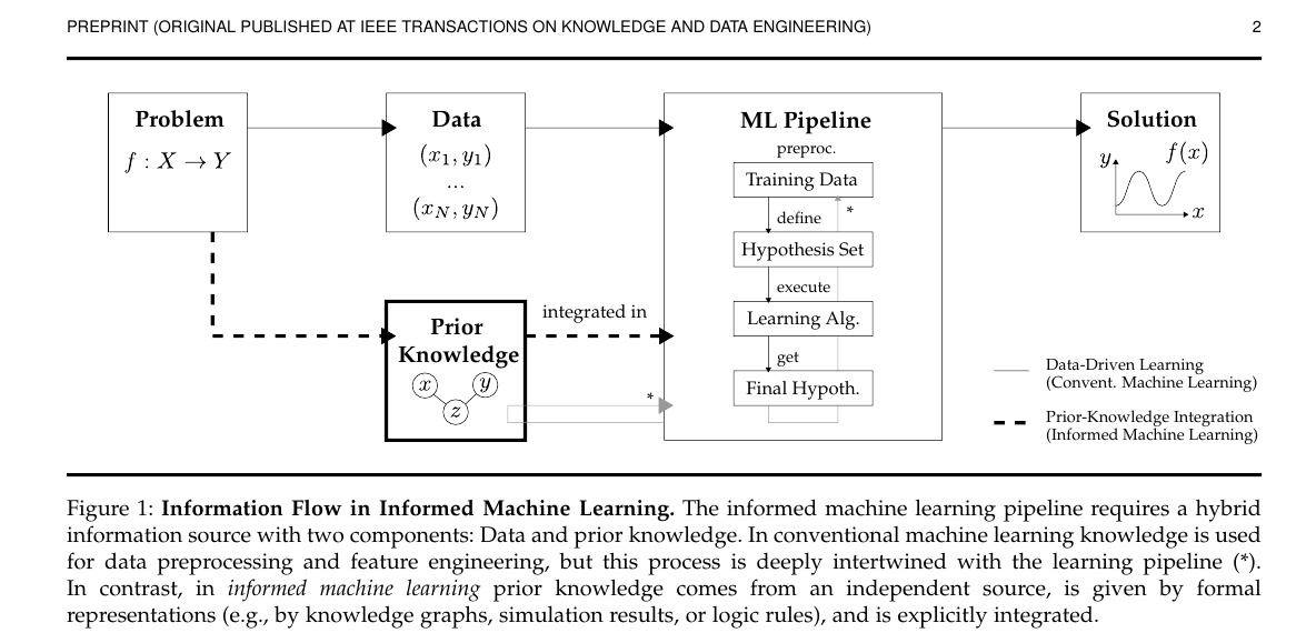
Role of the Figure

Figure 1 is not a method diagram; it is a conceptual diagram. It answers the following question:

Where exactly does informed machine learning differ in essence from ordinary machine learning?

Basic Structure of the Figure

The whole figure contains two input sources:

• Data
• Prior Knowledge

They jointly enter the ML Pipeline and eventually produce the Solution.

Conventional machine learning mainly relies on sample data:

• start from the problem definition
• collect training data
• define the hypothesis set
• run the learning algorithm
• obtain the final hypothesis f(x)

Informed machine learning adds an additional information source on top of this process:

• this information source is not directly inferred from the training samples
• it comes from the problem itself, scientific laws, world knowledge, expert experience, or human feedback
• and it must be explicitly connected to the pipeline in some formalized form

The Three Conditions This Figure Really Emphasizes

The authors are actually quite strict about what counts as prior knowledge. Not every kind of “experience” qualifies:

1. Independent source
   Prior knowledge is not directly fitted from the current training data; it comes from outside the data.

2. Formal representation
   The knowledge must be expressed in a machine-operable form, such as equations, rules, graph structures, simulation results, probabilistic relations, and so on.

3. Explicit integration
   The knowledge does not merely remain in the researcher’s mind, nor is it only used vaguely through feature engineering. It must enter the learning process explicitly.

How to Understand the Pipeline in This Figure

Inside the ML Pipeline, there are four core components:

• Training Data
• Hypothesis Set
• Learning Algorithm
• Final Hypothesis

The one worth remembering most carefully is Hypothesis Set.

It is not the final trained model. Rather, it is:

• the function space into which the model is allowed to fall
• the collection of model structures and inductive biases
• what kinds of solutions are allowed and what kinds are ruled out from the start

Accordingly, prior knowledge has three especially typical insertion points:

1. Into the training data
   For example, additional samples are generated through simulation.

2. Into the hypothesis set
   For example, rules, graph structure, or symmetry are directly encoded as architectural bias.

3. Into the learning algorithm
   For example, constraints are rewritten as a loss, a regularizer, or a training rule.

What This Figure Suggests for Reading Papers

When encountering an informed ML paper in the future, do not first ask “what network did it use?” Instead, ask:

1. Where does its prior knowledge come from?
2. In what form is that knowledge represented?
3. Is it injected into the data, the hypothesis set, or the learning algorithm?

These three questions are exactly the backbone of the taxonomy that follows.

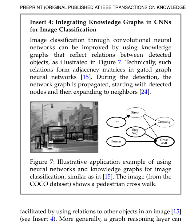
Table 4 Close Reading: How to Read the Taxonomy Path

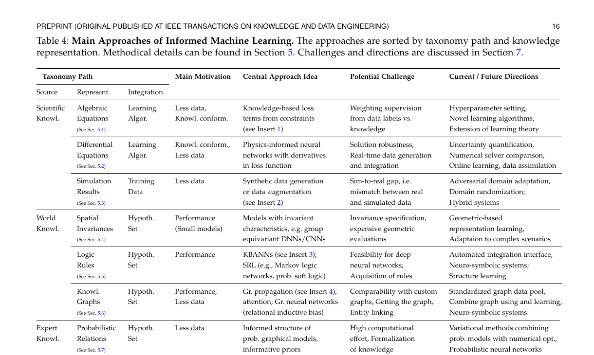
Role of the Table

Table 4 is the most practically useful summary table in the survey. It is not listing method names; it is listing “knowledge-integration paths.” Each row can be read as a three-part expression:

Source -> Representation -> Integration

That is:

• where the knowledge comes from
• what form the knowledge takes
• through which interface the knowledge enters the machine learning system

After these three columns, the authors add:

• Main Motivation
• Central Approach Idea
• Potential Challenge
• Current / Future Directions

This connects the entire chain: why the method appears, what it usually does, where the main difficulties lie, and where it is likely to go next.

A Useful Way to Read This Table

Do not treat it as a static classification table. Read each row as a complete sentence.

For example:

• Scientific Knowledge -> Algebraic Equations -> Learning Algorithm
  means that the knowledge comes from scientific laws, is represented as algebraic equations, and enters the learning algorithm through a loss or constraints.

• World Knowledge -> Logic Rules -> Hypothesis Set
  means that the knowledge comes from human understanding of regularities in the world, is represented as logic rules, and enters the model structure or hypothesis space.

• Scientific Knowledge -> Simulation Results -> Training Data
  means that the knowledge comes from a simulation system and ultimately enters the training set as samples or augmented data.

Once read this way, the taxonomy becomes a tool for understanding methods rather than a memory exercise in classification.

Row-by-Row Interpretation of Table 4

1. Scientific Knowledge -> Algebraic Equations -> Learning Algorithm

The main motivations for this family are:

• limited data
• or the need to ensure that model outputs conform to known scientific laws

The central idea is:

• write the knowledge as algebraic constraints
• then turn those constraints into loss terms or regularizers

The most typical way to understand this line is:

The model is not only asked to fit the labels, but is simultaneously penalized for violating known knowledge constraints.

The main challenge is:

• how to balance supervision from data against supervision from knowledge

This is exactly why many informed-loss methods end up requiring extensive hyperparameter tuning.

2. Scientific Knowledge -> Differential Equations -> Learning Algorithm

This line corresponds to the broad family of physics-informed neural networks.

The central idea is:

• the model should not only fit observations
• it should also satisfy a differential equation through its derivatives

This is stronger than ordinary algebraic constraints because:

• the constrained object is not a static variable relation
• but a relation among functions and their derivatives

The authors emphasize several key difficulties:

• robustness of the solution
• integration of real-time data
• comparison with classical numerical solvers

This means that PINNs are not “better simply because PDE loss is added”; they must be seriously compared with the numerical-analysis tradition.

3. Scientific Knowledge -> Simulation Results -> Training Data

This line does not directly turn knowledge into a loss. Instead, it first “unfolds” knowledge through a simulation system into data.

Therefore, it enters Training Data, not the Learning Algorithm.

Common forms include:

• synthetic data generation
• data augmentation
• simulator-generated labels

Its key challenge is the sim-to-real gap:

• simulated data differ from real data
• a model that performs well in simulation may fail in the real world

Accordingly, future directions often involve:

• domain adaptation
• domain randomization
• hybrid systems

4. World Knowledge -> Spatial Invariances -> Hypothesis Set

The knowledge here is:

• translation invariance
• rotation invariance
• invariance / equivariance under group actions

This kind of knowledge is not taught through extra supervision; it is directly encoded into the model structure.

That is why it enters the Hypothesis Set.

In one sentence:

Instead of forcing the model to learn invariance after training, the model is only allowed from the outset to learn within structures that already satisfy that geometric regularity.

The importance of this family lies in the fact that:

• it can often achieve better generalization with smaller models
• because the structural bias itself reduces the useless search space

5. World Knowledge -> Logic Rules -> Hypothesis Set

This is a particularly useful line within informed ML, and it also marks one of the core interfaces of neuro-symbolic learning.

The representative paths mentioned by the authors include:

• KBANN
• Statistical Relational Learning
• Markov logic networks
• probabilistic soft logic

The key point is:

• logic rules are not merely a training-time penalty
• they can also be mapped into network structure, inference structure, or feasible hypothesis space

There are two central challenges:

1. scalability in deep-network settings
2. where the rules themselves come from

The second point is especially important, because in real tasks rules are often not given in finished form; further structure learning is required.

6. World Knowledge -> Knowledge Graphs -> Hypothesis Set

This line represents relational knowledge in graph form.

Its core idea is typically:

• to use graph propagation, attention, or graph neural networks
• and inject relational structure among entities as relational inductive bias

This path is especially well understood as:

The graph is not an ordinary additional feature; it is a structural prior about who is related to whom and how relations propagate.

The main challenges are:

• graphs are often custom-built, making papers hard to compare
• the graph itself may be incomplete
• entity linking is difficult

Therefore the authors highlight the following directions:

• standardized graph resources
• combining graph usage with graph learning
• stronger neuro-symbolic integration

7. Expert Knowledge -> Probabilistic Relations -> Hypothesis Set

Here the prior knowledge is not a hard logical constraint, but probabilistic relations, structural dependencies, or informative priors supplied by experts.

Such methods are common in:

• probabilistic graphical models
• Bayesian priors
• variational approaches

The core logic is:

• do not first interpret the knowledge as “must be satisfied”; instead, interpret it as “certain structures or parameters are more likely to occur” Its main difficulties are:

• high computational cost

• difficulty of formalizing expert knowledge

8. Expert Knowledge -> Human Feedback -> Learning Algorithm

This line can be read as:

• human feedback can itself serve as prior knowledge
• but it usually enters as part of the training process rather than as a static structure

Therefore it more often enters the Learning Algorithm than the Hypothesis Set.

The typical forms listed by the authors include:

• HITL reinforcement learning
• explanation alignment
• visual analytics / interactive machine learning

The difficulties here are very concrete:

• human feedback is slow
• human intuition is difficult to formalize
• evaluation protocols are unstable

What These Two Figures Together Reveal as the Real Framework of the Survey

Figure 1 provides the conceptual framework:

• informed ML = data + independently available prior knowledge

Table 4 provides the operational framework:

• Source
• Representation
• Integration

In other words, what this survey truly establishes is not a “list of methods,” but an analytical coordinate system:

1. First determine the source of knowledge.
2. Then determine the representation of that knowledge.
3. Then determine where it enters the pipeline.
4. Finally analyze its motivation, method, challenges, and future directions.

Condensed Takeaways Worth Retaining

For my current reading, this survey can be condensed into the following four points:

1. The essence of informed ML is not “having experience,” but having prior knowledge that comes from an independent source, is formalizable, and can be explicitly integrated.
2. Any method can be located using Source -> Representation -> Integration.
3. Scientific knowledge more often enters the Learning Algorithm, world knowledge more often enters the Hypothesis Set, and simulation-based knowledge more often enters Training Data.
4. The value of this survey is not that it provides one unified model, but that it provides one unified way of reading the field.

Questions Worth Pursuing After Reading

1. Which knowledge representations can be transformed into one another, such as rules, graphs, and probabilistic relations?
2. What is the essential difference between placing the same knowledge in the Hypothesis Set versus the Learning Algorithm?
3. When data and knowledge conflict, which should the system trust more?
4. Where are the boundaries between informed ML and neuro-symbolic learning, physics-informed learning, and causal learning?

Section 4 Close Reading: Taxonomy Is Not a Static Classification Table but a Navigation Map

Where This Section Sits in the Overall Survey

The role of Section 4 is not to enumerate method details, but to abstract into a unified framework the recurring patterns that the authors observed throughout the literature.

In other words:

• Section 2 answers “what counts as informed ML”
• Section 3 answers “how this taxonomy was distilled from the survey”
• Section 4 answers “what dimensions and elements the taxonomy itself contains”
• only in Section 5 do concrete methods get placed into the taxonomy

So if Section 5 feels crowded and scattered, that usually does not mean the methods themselves are chaotic; it means Section 4 has not yet been fully digested.

The Three Main Axes of the Taxonomy

The authors decompose the method space of informed ML into three dimensions:

1. Knowledge Source
2. Knowledge Representation
3. Knowledge Integration

These correspond to three questions:

1. Where does the prior knowledge come from?
2. In what form is it expressed?
3. At which point in the machine learning pipeline is it integrated?

Among these three axes, the authors actually emphasize the second one most: representation.

This is because:

• source is more about application background
• integration is more about the method interface
• representation is the actual bridge between the two

That is, whether knowledge can be absorbed by a machine learning system depends not only on whether knowledge exists, but on what form that knowledge takes.

Knowledge Source: The Three-Way Split Is Not Mainly About Discipline but About Degree of Formalization

Section 4.1 divides knowledge sources into:

• Scientific Knowledge
• World Knowledge
• Expert Knowledge

These three categories are easy to misread as a simple disciplinary partition, but what the authors really want to express is a spectrum:

• from more formal, explicitly validated knowledge
• to more general but often implicitly validated world knowledge
• to more experience-driven and intuitive expert knowledge

So this is not a strict ontology, but a practical classification.

The authors explicitly acknowledge that:

• these categories are not exhaustive
• and they are not fully disjoint

Their main purpose is to identify common paths of knowledge integration.

Knowledge Representation: The Core Interface of the Taxonomy

Section 4.2 is the most critical part of the entire taxonomy.

The authors extract eight common representation types:

• algebraic equations
• differential equations
• simulation results
• spatial invariances
• logic rules
• knowledge graphs
• probabilistic relations
• human feedback

One especially important judgment here is:

The authors are not trying to construct the mathematically minimal set of representation types; they are preserving the representations that most commonly appear in the literature and are closest to practice.

That is why:

• differential equations are listed separately instead of being folded back into algebraic equations
• simulation results are also listed separately instead of being treated merely as the output of an equation solver

The reason is not that these forms cannot be transformed into each other, but that they often correspond to different machine learning interfaces.

The Eight Representation Types Can Be Memorized as Three Groups

First group: scientific-law-type

• algebraic equations
• differential equations
• simulation results

This group usually serves either to make the model conform to scientific laws or to supplement data through simulation.

Second group: symbolic-and-structural

• spatial invariances
• logic rules
• knowledge graphs

This group usually serves structural bias, relational modeling, or interpretable constraints.

Third group: uncertainty-and-interaction

• probabilistic relations
• human feedback

This group usually deals with expert experience, intuition, incomplete knowledge, and human-machine interaction.

This grouping is a more stable memory aid than simply memorizing eight isolated labels.

Knowledge Integration: Knowledge Does Not Only Enter Through Loss

The value of Section 4.3 is that it splits “knowledge entering the model” into four possible locations:

• Training Data
• Hypothesis Set
• Learning Algorithm
• Final Hypothesis

Many people hear “informed ML” and immediately think “add a knowledge loss.” That is only one possibility, and only the Learning Algorithm column.

What the authors want to show is:

• knowledge can be used to create data
• knowledge can constrain the model space
• knowledge can modify the training rule
• knowledge can even be used after training to validate or refine the final output

The Two Most Common Locations

Although all four locations are possible, the authors clearly state that most papers concentrate on two central stages:

• Hypothesis Set
• Learning Algorithm

This also matches actual reading experience:

• structural-bias methods often encode knowledge into architecture / graph / kernel / rule structure
• constraint-optimization methods often encode knowledge into loss / regularization / constrained optimization

Figure 2 Shows Not Only the Taxonomy but the Taxonomy Plus Literature Frequency

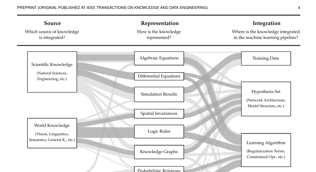
Figure 2 is easy to see as an ordinary classification diagram, but it actually overlays survey findings:

• the size of each block reflects its relative frequency in the literature
• the width of each Sankey path reflects how often a particular combination occurs
• darker paths indicate the main paths emphasized by the authors

This is important because it means:

This is not the space of all logically possible methods, but the method space that has already been repeatedly practiced in the literature.

Therefore the figure has two uses:

1. as an entry map for newcomers
2. as a baseline / gap-analysis tool for researchers

Two Directions for Reading the Taxonomy

In Section 4, the authors make a very useful observation that is easy to overlook:

• application-oriented readers may prefer to read from left to right
• method-oriented readers may prefer to read from right to left

That is:

Reading Left to Right

If one starts with a knowledge source, for example:

• physical equations
• medical graphs
• linguistic rules

then the natural questions are:

• what representation is most suitable?
• through which interface should it be injected?

Reading Right to Left

If one starts with a method, for example:

• constrained optimization
• graph neural networks
• teacher-student distillation

then the reverse questions become:

• what types of representation fit this interface best?
• from what kinds of knowledge source do those representations usually come?

This perspective is especially useful for topic selection.

An Empirical Pattern in Section 4: Different Sources Often Prefer Different Representations

At the junction of Section 3.2 and Section 4, the authors repeatedly emphasize an empirical regularity:

• Scientific Knowledge often goes toward equations / simulations
• World Knowledge often goes toward logic rules / graphs / invariances
• Expert Knowledge often goes toward probabilistic relations / human feedback

This is not an absolute rule, but it suggests that the “character” of the knowledge source influences the form it is naturally suited to.

The point most worth remembering is:

informed ML is not “first choose one universal method and then stuff every kind of knowledge into it”; rather, different knowledge types are naturally biased toward different interfaces.

The Relation Between Section 4 and Table 2 / Table 3

Section 4 provides the conceptual taxonomy.
Table 2 and Table 3 provide the observed cross-distributions from the survey.

This can be understood as follows:

• Section 4 tells you what the axes are
• Table 2 tells you how source and representation tend to pair
• Table 3 tells you how representation and integration tend to pair

So the survey is not just giving one big figure. It actually provides three layers of information:

1. conceptual framework
2. empirical frequency
3. representative main paths

My Summary of Section 4

The real contribution of Section 4 is not that it invents a few classification names, but that it reorganizes informed ML from a collection of scattered methods into a navigable method space.

This can be compressed into one note:

The significance of the taxonomy is not that it archives papers, but that it decomposes the question “how does knowledge enter a learning system?” into the three analyzable interfaces of source, representation, and integration.

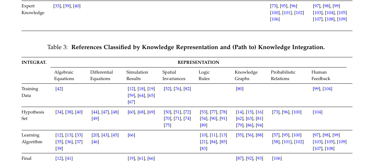
Section 5.5 Close Reading: What the Logic Rules Route Is Really Doing

Why Logic Rules Occupy Such an Important Position in the Survey

Among all representation types, logic rules are the closest to traditional symbolic AI.

Their importance lies in the fact that:

• they preserve explicit semantic relations
• they can interface with learning systems in multiple ways
• they are one of the most direct points of contact between informed ML and neuro-symbolic learning

In other words, logic rules are not a peripheral representation type, but a very central informed ML path.

5.5.1: Logic Rules Most Commonly Come from World Knowledge

The authors say that logic rules can come from multiple sources, but the most common one is World Knowledge.

The survey gives several representative examples:

• object-property rules
  for example, animals that fly and lay eggs are more likely to be birds

• object-relation rules
  for example, certain characters often co-occur in game scenes

• linguistic rules
  for example, when a sentence contains but, the sentiment after it dominates; or citation-tag order constraints

• social / relational dependency rules
  for example, authors who cite each other are more likely to belong to related research fields

These examples together show one key fact:

A logic rule is particularly well suited to expressing relational knowledge among discrete objects.

Unlike equations, it does not emphasize continuous numerical relations. Instead, it emphasizes:

• if-then structure
• co-occurrence
• implication
• symbolic dependency

5.5.2: Logic Rules Mainly Follow Two Integration Routes

A central observation in this subsection is:

• logic rules often enter the Hypothesis Set
• and secondarily the Learning Algorithm

That is, rules either reshape the model structure or reshape the training objective.

Although both are called “rule injection,” they are fundamentally different.

Route A: Injecting Rules into the Hypothesis Set

1. The Deterministic Route: KBANN / Neural-Symbolic Architecture

A representative method here is KBANN.

Its core idea is not:

• first train an ordinary network
• then use rules as a post-processing step

Rather, it is:

• directly translate rules into network structure and initial weights

Insert 3 decomposes this process into four steps:

1. obtain the rules and rewrite them hierarchically if needed
2. map the rules to the network architecture
3. add hidden nodes not explicitly given in the rules
4. perturb the entire set of weights and continue learning

A concise way to retain the distinction is:

KBANN is not “rules as a regularizer”; it is “rules first shape the network, and data then refine the network.” So it embodies a strong structural prior.

2. The Probabilistic Route: SRL / MLN / PSL

Another way of placing rules into the hypothesis set is not through deterministic structure but through probabilistic structure.

The authors place this line under statistical relational learning.

Representative frameworks include:

• Markov Logic Networks
• Probabilistic Soft Logic

The basic idea is:

• first-order logic rules are no longer treated as hard constraints that must be strictly satisfied
• but as templates that define probabilistic dependencies

That is, the rules determine:

• which random variables are related
• which joint configurations are more likely
• how satisfying a rule increases probability mass on certain states

This step is crucial because it connects:

• symbolic rule
• probabilistic uncertainty

Thus this line can be understood as:

Rules no longer operate only at the level of “true / false,” but shape the hypothesis space at the level of “more likely / less likely.”

Route B: Injecting Rules into the Learning Algorithm

The biggest difference here is:

• the model structure itself may not be directly determined by the rules
• but the training objective is constrained by them

The authors mention semantic loss as a representative family.

The core idea is:

• turn logic rules into a differentiable penalty term
• then add that term into the objective function

The survey mentions several technical interfaces:

• use t-norm to relax logic rules into continuous form
• derive semantic loss from first principles using a set of axioms

The significance of this route is:

The rules are preserved, but the model can still remain a standard deep learning architecture instead of being completely rewritten.

So it is often more flexible and easier to embed into existing pipelines.

Why the Teacher-Student Line Deserves to Be Remembered Separately

Section 5.5 also highlights another useful variant:

• first integrate rules on the teacher side
• then let the student imitate the teacher

This idea matters because it suggests that rules do not have to directly constrain the final deployed model itself.

They can also:

• constrain a stronger, more “knowledge-heavy” teacher first
• then transfer the knowledge to the student through distillation

This is exactly the typical logic behind works like LogicNet.

So from the perspective of your toy projects:

• logic_net_toy is closer to rules -> learning algorithm -> teacher-student
• semantic_loss_toy is closer to rules -> learning algorithm -> differentiable constraint

Whereas KBANN is another distinct branch:

• rules -> hypothesis set -> architecture design

All three belong to the logic-rules route, but they are not the same kind of method.

What Is Most Easily Confused Within the Logic-Rules Literature

At the surface level, logic-rule methods all look like attempts to “make the model obey rules.” But in reality they operate on at least three different levels:

1. Structural level
   rules shape the model structure or feasible hypothesis space, as in KBANN

2. Probabilistic level
   rules define dependency templates among random variables, as in MLN / PSL

3. Optimization level
   rules become differentiable penalties during training, as in semantic loss

If these three levels are not kept separate, the logic-rule literature easily turns into an undifferentiated mixture.

The Authors’ Judgment on the Logic-Rules Route

In Section 7, the authors identify two core challenges for logic rules:

1. can this route still scale efficiently in the era of deep neural networks?
2. if rules are not given in advance, where do they come from?

The first question corresponds to:

• scalability
• automated interfaces for knowledge integration
• more realistic neuro-symbolic systems

The second corresponds to:

• rule acquisition
• structure learning

In other words, the real difficulty of the logic-rules route is not only “how to use rules,” but also “how rules are obtained, maintained, and updated.”

My Summary of Section 5.5

The logic-rules route is not one single method family, but an entire collection of interfaces for connecting symbolic rules to learning systems.

It can be compressed into one note:

The fundamental value of logic rules is not merely that they provide constraints, but that they turn discrete relational knowledge into computable structural bias, probabilistic dependence, or optimization signals.

Section 5.6 Close Reading: What the Knowledge Graphs Route Is Really Doing

Why Knowledge Graphs Form a Distinct Main Line in Informed ML

Knowledge graphs are easy to misread as another notation for logic rules. The authors separate them out for a clear reason.

Logic rules emphasize:

• propositional relations
• implication structure
• if-then constraints

Knowledge graphs emphasize:

• entities
• relations
• graph connectivity structure

So the core of graphs is not “whether a rule holds,” but:

how objects in the world are connected to one another, and how that relational structure can be used as relational inductive bias by the model.

That is why knowledge graphs in this survey are not merely a data resource, but a distinct type of knowledge representation.

5.6.1: Graphs Most Often Come from World Knowledge, but Not Only from World Knowledge

In 5.6.1 the authors first emphasize:

• graph is a highly general modeling tool
• in principle it can represent many kinds of structured knowledge

But in the surveyed literature, the most common source is still World Knowledge.

World Knowledge

The authors’ representative examples are very telling:

• Visual Genome
  turns object attributes and object relations in natural images into a graph

• ConceptNet
  turns everyday commonsense concepts and relations into a graph

• WordNet
  turns semantic and lexical relations among words into a graph

Together these examples show:

Graphs are particularly suited to expressing “what entities are related to what,” rather than “what propositional constraint must hold.” This is the root difference between graphs and logic rules.

This is especially clear in language tasks:

• rules look more like local syntactic / semantic constraints
• graphs look more like concept networks, lexical networks, or knowledge-base structure

Scientific Knowledge

The authors also emphasize that graphs are not only for commonsense knowledge bases.

In scientific settings, graphs can directly represent structured systems, such as:

• spring-coupled masses in physical systems
• gene-protein interaction networks in medicine
• hierarchical diagnostic systems such as ICD

This means:

Graph is not a “natural-language knowledge-base-only” format, but a general-purpose representation of relational structure.

Whenever objects and relations are central, graph becomes a natural interface.

5.6.2: Knowledge Graphs Can Enter Almost Every Part of the Pipeline

The observation worth remembering most in this subsection is:

• knowledge graphs appear in all four integration locations
• but the most prominent one is still the Hypothesis Set

This is somewhat similar to logic rules, but the graph route focuses more on relational structural bias than on rule constraints.

Route A: Graphs Enter the Hypothesis Set

This is the path the authors regard as most central.

1. Graph Neural Networks as Relational Structural Bias

The authors explicitly interpret methods like GNNs as:

• models whose architecture already assumes that the world is composed of interrelated objects

In other words, graph enters the hypothesis set not as “add one graph constraint,” but as:

• organize the computation itself around nodes and edges

This is what the survey refers to as relational inductive bias.

One can understand it as:

From the beginning, the model does not treat samples as isolated vectors, but as entities and relations inside a graph.

2. Explicitly Connecting an External Knowledge Graph as a Second Information Source

Besides “the model itself is graph-structured,” there is an even stronger design:

• an external knowledge graph already exists
• and it is connected to the network as an additional information source

In this case the graph is not only inductive bias; it becomes a genuine second source of knowledge.

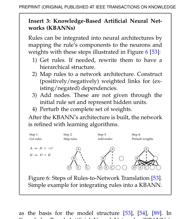
The image-classification example in Insert 4 is easy to understand:

• objects are first detected in the image
• the relations among objects are given by the knowledge graph
• graph propagation starts from the detected nodes and expands to neighbors
• semantic relations among objects help disambiguate the current object

For example, in a street scene:

• person
• crosswalk
• stop sign
• street

Each object alone may be ambiguous, but within one relational graph the judgment becomes much stronger.

3. The Significance of a Graph Reasoning Layer

The authors also mention a more general notion:

• graph reasoning layer

Its idea is:

• insert an additional graph-propagation layer into some existing neural layer
• enhance the representation through a knowledge graph

This means graph integration does not necessarily require the entire model to be a GNN end-to-end.

A more common realistic scenario may be:

• the backbone remains CNN / Transformer / MLP
• and only a graph-based reasoning module is inserted in the middle

This is important in engineering terms because it is easier to combine with existing models.

Route B: Graphs Enter the Training Data

This route is especially prominent in the graph literature, and the keyword highlighted by the authors is distant supervision.

The basic idea is:

• use entity relations from a knowledge graph to automatically annotate text
• thereby generate training samples

The most naive form is:

• if a sentence contains a pair of entities already known to be related in the graph
• treat that sentence as a training sample

But this introduces substantial noise, so later work uses attention and related mechanisms to reduce the impact of noisy samples.

This route can be interpreted as follows:

A knowledge graph does not have to enter the model directly; it can first be turned into weak supervision and enter the training data.

This is somewhat analogous to simulation results:

• both can first “unfold” knowledge into trainable samples

The difference is that graph-based unfolding usually produces automatic labels or distant supervision rather than simulated data.

Route C: Graphs Enter the Learning Algorithm

The authors mention two especially memorable families.

1. Graph Laplacian Regularization

This is the classical idea of graph regularization:

• variables that are close on the graph should behave more similarly in the model
• variables that are unconnected can vary more freely

Such methods are common in:

• bioinformatics
• pathway-information integration

Its essence is:

The graph structure is translated into an optimization preference rather than directly translated into model structure.

2. Knowledge-Graph-Enhanced Embedding / Language-Model Training

Another family uses graph relations as extra context during the training of word embeddings or language models.

For example:

• use graph-based lexical relations to enrich the context of word2vec
• use knowledge-graph embeddings to support the training of models like ERNIE / BERT

This suggests that when graph enters the learning algorithm, it often plays the role of:

• a source of regularization
• a source of additional context
• a source of semantic supplementation for representation learning

Route D: Graphs Enter the Final Hypothesis

This route is easy to overlook, but it has real practical value.

The authors mention several representative examples:

• post-process word embeddings using knowledge graphs
• validate semantic segmentation in autonomous driving using street-map graphs
• refine predicted probabilities in object detection using graph consistency

This means that graph does not have to participate in training.

It can also serve after training as:

• consistency checking
• result refinement
• knowledge-based validation

From the perspective of safety and trustworthy AI, this route is especially important.

The Key Difference Between Knowledge Graphs and Logic Rules

These two routes are easy to mix up, but it is best to separate them sharply.

Logic Rules Are More Like:

• “if A and B, then C”: focused on propositional constraints and logical satisfiability

Knowledge Graphs Are More Like:

• “A has some relation to B”: focused on entity networks and relation propagation

Therefore:

• logic rules more naturally lead to semantic constraints, teacher-student distillation, and rule templates
• knowledge graphs more naturally lead to graph propagation, graph attention, GNNs, and entity linking

Of course, the two can approach each other:

• graph edges can imply rules
• rules can also be converted into graph structure

But in this survey they are classified separately because the center of gravity of their machine-learning interfaces is different.

The Authors’ Judgment on the Knowledge-Graph Route

In Section 7, the authors’ summary of knowledge graphs is especially clear.

There are three main challenges:

1. Different papers use different graphs, so methods are difficult to compare
   Many works begin from templates such as ConceptNet or Visual Genome, but then apply extensive custom modifications.

2. Getting the graph itself is difficult
   This is exactly what the authors call Getting the graph.

3. Entity linking is difficult
   Especially when the model must align entities in text or images to nodes in the graph, this step often becomes the bottleneck.

The corresponding future directions include:

• building standardized graph pools / benchmarks
• combining graph usage with graph learning
• continuing toward neuro-symbolic systems

The single most important point to remember here is:

The real difficulty of knowledge graphs often lies not in “how to write the graph network,” but in where the graph comes from, how good the graph is, and how graph nodes align with the objects of the current task.

My Summary of Section 5.6

The core of the knowledge-graph route is not simply “use a graph model,” but to treat relational structure as a second information source or a structural bias inside the learning system.

This can be compressed into one note:

The essential value of a knowledge graph is that it turns an entity-relation network into relational structure that the model can exploit to improve representation, training, or result validation.

Logic Rules vs Knowledge Graphs: Comparative Notes

Why These Two Routes Must Be Compared Explicitly

In the informed ML literature, logic rules and knowledge graphs are often placed together under “symbolic / structured knowledge.” But if they are not carefully separated, two misunderstandings easily arise:

1. treating a graph as “a rule in different clothing”
2. treating a rule as “just one kind of edge in a graph” Neither view is accurate enough.

A better understanding is:

• logic rules answer “which propositional relations ought to hold”
• knowledge graphs answer “which entities are related, and how that relational structure propagates” So although both are structured knowledge, their interface focus differs.

One-Sentence Distinction

The shortest version to remember is:

• logic rules are more like constraints
• knowledge graphs are more like structure

With one further step of detail:

• the core semantic unit of logic rules is proposition, condition, and implication
• the core semantic unit of knowledge graphs is entity, relation, and connectivity pattern

Comparison 1: The Basic Unit of Knowledge Is Different

Logic Rules

Its basic units are usually:

• propositions
• predicates
• logical relations
• if-then structures

Typical forms look like:

• A and B -> C
• “if a sentence contains but, then the sentiment after it dominates”

• “if an object flies and lays eggs, it is more likely to be a bird” The emphasis here is:

• when the condition holds, the conclusion should be supported or satisfied

Knowledge Graphs

Its basic units are usually:

• entity nodes
• relation edges
• local neighborhoods
• global connectivity structure

Typical forms look like:

• (Mario, appears_with, Peach)
• (word, synonym_of, another_word)
• (gene_a, interacts_with, gene_b)

The emphasis here is:

• who is related to whom
• how those relations are organized across the graph

Comparison 2: What They Want the Model to Learn Is Different

Logic Rules Want the Model to Learn:

• to satisfy certain logical constraints
• not to violate certain discrete rules
• to maintain some kind of symbolic consistency in reasoning

So this line is more about:

• consistency
• constraint satisfaction
• rule-guided reasoning

Knowledge Graphs Want the Model to Learn:

• to exploit relational structure among objects
• to use neighbors and paths to enrich representations
• to propagate evidence through a relation network

So this line is more about:

• relational reasoning
• context enrichment
• structure-aware representation learning

Comparison 3: The Most Common Integration Locations Are Different

Logic Rules

In the survey, the most common locations are:

• Hypothesis Set
• Learning Algorithm

That is:

• rules shape structure
• or rules enter the loss / optimization

Representative interfaces:

• KBANN
• MLN / PSL
• semantic loss
• teacher-student rule distillation

Knowledge Graphs

In the survey, all four locations appear, but the most prominent one remains:

• Hypothesis Set

In addition, the following are also common:

• Training Data
• Learning Algorithm
• Final Hypothesis

Representative interfaces:

• GNN
• graph reasoning layer
• graph attention
• distant supervision
• graph Laplacian regularization
• knowledge-based validation

In one sentence:

Rules more often “constrain the model,” whereas graphs more often “reconstruct the way the model sees the world.”

Comparison 4: The Typical Method Families Are Different

Common Logic-Rules Families

1. KBANN
   rule -> network structure

2. MLN / PSL / SRL
   rule -> probabilistic dependency template

3. semantic loss
   rule -> differentiable constraint term

4. teacher-student
   rule -> teacher guidance -> student imitation

Common Knowledge-Graph Families

1. GNN / graph propagation
   graph structure -> relational inductive bias

2. graph reasoning layer
   insert graph propagation into an existing backbone

3. graph attention
   use graph neighborhoods to enhance representation or feature selection

4. distant supervision
   graph relations -> automatic annotation -> training data

5. graph regularization
   graph Laplacian-type constraints -> learning algorithm

6. knowledge-based validation
   graph consistency -> posterior correction or result validation

Comparison 5: The Kinds of Knowledge They Best Express Are Different

Scenarios Better Suited to Logic Rules

When knowledge naturally looks like the following, rules are usually more natural:

• “if …, then …”
• “these cannot hold simultaneously”
• “some discrete constraint must be satisfied”
• “labels have exclusion / implication / ordering relations”

• “the explanation must satisfy some satisfiability structure” Typical tasks include:

• label constraints

• logical reasoning
• structured-output constraints
• rule templates in weak supervision
• symbolic rules in sentiment / sequence tagging

Scenarios Better Suited to Knowledge Graphs

When knowledge naturally looks like the following, graphs are usually more natural:

• “who is related to whom”
• “objects participate in multiple kinds of relations”
• “neighbors, paths, and local context must be exploited”
• “concepts and entities form a network”

• “extra evidence must be propagated through relations” Typical tasks include:

• object relations in images

• entity / concept networks in NLP
• recommendation / knowledge-base QA
• biomedical interaction networks
• any task involving many entities, many relations, and contextual propagation

Comparison 6: The Main Failure Modes Are Different

Major Difficulties for Logic Rules

1. Where do the rules come from?
   In many tasks, rules are not given in finished form.

2. How are the rules formalized?
   It is not easy to turn natural-language experience into logical form.

3. What if rules conflict with data?
   Data noise, knowledge noise, and incompleteness can all create conflict.

4. How scalable are the rules?
   In deep networks, rule injection is not always stable or efficient.

Major Difficulties for Knowledge Graphs

1. Where does the graph come from?
   This is exactly the survey’s getting the graph.

2. How good is the graph?
   The graph may be incomplete, outdated, sparse, or mismatched to the task.

3. Is entity linking reliable?
   Whether input objects can be aligned correctly to graph nodes is often the main bottleneck.

4. Why are different methods hard to compare?
   Because each paper often customizes its graph resource.

Comparison 7: They Interface with Differentiable Learning Systems in Different Ways

When Logic Rules Enter Differentiable Systems

What typically needs to happen is:

• discrete logic must be relaxed into continuous form
• rule satisfaction must become a loss
• rule templates must be mapped into structure or probabilistic terms

That is, when rules enter neural systems they often undergo a transition from “discrete” to “learnable interface.”

When Knowledge Graphs Enter Differentiable Systems

What typically needs to happen is:

• the graph becomes a message-passing structure
• adjacency relations become attention / propagation / regularization
• nodes and edges become continuous embeddings

That is, graphs are more naturally “structural” from the start, and therefore connect more directly to neural representation learning.

Comparison 8: The Two Are Not Opposed; They Can Work Together

Although they differ, in many tasks they can naturally be combined.

A common division of labor is:

• use the graph to provide the relational backbone among entities
• use rules to specify which inferences or outputs are acceptable

That is:

• the graph provides the relational background
• the rule provides the inferential constraint

Going one step further:

• edge types in a graph may induce rules
• rules may help filter valid relations in a graph

So the more accurate statement is not “rule versus graph, choose one,” but:

When knowledge contains both a relational network and symbolic constraints, the two should often cooperate with different roles.

Four Very Practical Questions for Choosing a Method

When reading a paper and trying to quickly determine which route it belongs to, ask four questions:

1. Is the core of the knowledge expressing “constraints,” or expressing a “relation network”?
2. Is the model mainly “satisfying rules,” or “using neighbors and connectivity structure”?
3. Is the main interface loss / constraint, or propagation / attention / graph architecture?
4. If the graph were removed, or if the rule were removed, would the model lose structural context or logical consistency?

These four questions are usually sufficient to locate the paper quite clearly.

How This Relates to Your Current Reading Path

Given your current path, this comparison is especially useful:

• LogicNet
  more clearly belongs to the logic-rules route, with the emphasis on rules -> teacher/student -> learning algorithm

• Semantic Loss
  also belongs to the logic-rules route, with the emphasis on rules -> differentiable constraint

• Knowledge Graph-oriented work
  usually leans more toward relations / propagation / graph-enhanced representation than toward logical satisfiability itself

This means that when you later read graph-based papers, you should not first ask “what rule does it use?” Instead, ask:

• how are entities and relations defined?
• how does the graph enter the model?
• is the graph propagating information, or constraining outputs?

Final Compressed Memory Aid

The shortest contrast is:

• Logic Rules: propositional constraints, if-then structure, rule consistency, loss / architecture / probabilistic template
• Knowledge Graphs: entity relations, graph structure, neighborhood propagation, GNN / attention / validation

Compressed into one sentence:

Rules are more like “telling the model what it must not get wrong,” while graphs are more like “telling the model who is related to whom.”

Bridging Understanding: How Section 4, 5.5, and 5.6 Fit Together

If Figure 1, Figure 2, Table 4, and the discussions of logic rules and knowledge graphs are considered together, a very clear hierarchy emerges:

1. Figure 1 says that the essence of informed ML is “data + independently available prior knowledge.”
2. Section 4 says that this prior knowledge can be systematically classified via Source -> Representation -> Integration.
3. Section 5.5 unfolds Logic Rules to show how symbolic rules become structural bias or training constraints.
4. Section 5.6 unfolds Knowledge Graphs to show how relational structure becomes graph propagation, graph attention, graph regularization, or result validation.

So:

• Section 4 provides the method space
• Section 5.5 and 5.6 provide two detailed case studies of symbolic / relational routes

That is why reading the survey becomes much easier if the taxonomy is digested first, and then logic rules and knowledge graphs are read separately.

Compressed Version Worth Keeping in Mind

Section 4

• The taxonomy is not a static classification table; it is a navigation coordinate system for informed ML.
• Representation is the mediating interface between application knowledge and learning algorithms.
• Only by combining source, representation, and integration can one truly locate an informed ML method.

Section 5.5

• Logic rules are one of the most central symbolic knowledge representations in informed ML.
• Rules can reshape model structure, reshape the training objective, or define probabilistic dependencies.
• KBANN, MLN / PSL, and semantic loss / teacher-student are three different levels of the logic-rules route.

Section 5.6

• Knowledge graphs are one of the most central relational-structure representations in informed ML.
• Graphs can enter training data, hypothesis set, learning algorithm, and final hypothesis, though the most common location is the hypothesis set.
• Graph propagation, graph attention, GNNs, distant supervision, graph Laplacian regularization, and knowledge-based validation are the key interfaces on this route.