Citation and Scope
- Paper: A Semantic Loss Function for Deep Learning with Symbolic Knowledge (Xu et al., ICML 2018)
- In this note,
Semantic Lossrefers specifically to the 2018 formulation in which a propositional constraint $\phi$ is converted into a trainable loss through the total probability mass of its satisfying Boolean assignments.
This note places the paper in the following reading path:
Hu et al. 2016:rule -> teacher distribution -> studentSemantic Loss:rule -> exact semantic loss -> parameter updateDL2:constraint language -> differentiable surrogate / feasible set -> training + querying
The main contribution is therefore not simply that logic appears in training, but that:
- no teacher distribution is introduced;
- no local soft-truth score is used as the central objective;
- the optimization target is the exact probability mass of satisfying worlds.
Problem Setting
Let the training set be $$ \mathcal D=\{(x_n,y_n)\}_{n=1}^N. $$
For an input sample $x$, the network outputs a collection of Boolean variables $$ X=(X_1,\dots,X_m), $$ with an independent Bernoulli parameterization $$ p=(p_1,\dots,p_m),\qquad p_i=P(X_i=1\mid x). $$
The output space is the Boolean cube $$ \mathcal X=\{0,1\}^m. $$
For a concrete Boolean assignment $$ \mathbf b=(b_1,\dots,b_m)\in\{0,1\}^m, $$ its probability under the current network is $$ P_p(\mathbf b)=\prod_{i:b_i=1}p_i\prod_{i:b_i=0}(1-p_i). $$
Three points are worth keeping explicit:
Bernoullimeans that each $X_i$ is a binary random variable.Probability vectormeans that the network outputs one probability per bit, rather than one categorical distribution over classes.Independentmeans that the probability of a full Boolean world is constructed multiplicatively from the bitwise marginals.
Independent Bernoulli vs. Softmax
This distinction is essential for understanding why the exactly-one constraint is meaningful here.
If the final layer uses softmax with logits $$ z=(z_1,\dots,z_m)\in\mathbb R^m, $$ then the output is $$ \pi_i=\frac{e^{z_i}}{\sum_{j=1}^m e^{z_j}}, \qquad i=1,\dots,m, $$ with $$ \pi_i>0,\qquad \sum_{i=1}^m \pi_i=1. $$
This parameterizes a single categorical variable $$ Y\in\{1,\dots,m\}, \qquad \pi_i=P(Y=i\mid x), $$ so the “choose exactly one class” structure is already built into the architecture.
By contrast, Semantic Loss in this setting assumes $m$ Boolean output bits. The network may assign nontrivial probability to many invalid worlds, and the logical constraint must explicitly suppress them.
exactly-one and One-Hot Legal Worlds
For Boolean outputs
$$
X=(X_1,\dots,X_m),\qquad X_i\in\{0,1\},
$$
the Its arithmetic meaning is
$$
\sum_{i=1}^m b_i=1,\qquad b_i\in\{0,1\}.
$$ The satisfying worlds are precisely the one-hot Boolean assignments. For $m=4$, they are
$$
(1,0,0,0),\ (0,1,0,0),\ (0,0,1,0),\ (0,0,0,1).
$$ This is not the same object as a softmax probability vector. Here, a one-hot vector is a concrete Boolean world in the output space, not a probability distribution over classes. If softmax is imposed from the outset, the semantic content of If training relies only on standard supervision, the objective is typically written as
$$
\min_\theta \frac1N\sum_{n=1}^N \ell\bigl(y_n,p_\theta(\cdot\mid x_n)\bigr).
$$ For classification, the single-example loss is often
$$
\ell\bigl(y_n,p_\theta(\cdot\mid x_n)\bigr)
=
-\log p_\theta(y_n\mid x_n).
$$ This objective only requires the model to fit observed labels on labeled examples. It does not directly require logical consistency over the entire output space. As a result, standard supervision alone does not force the model to learn statements such as: This is precisely where Semantic Loss enters: even when labels are unavailable, a known logical constraint $\phi$ can still provide training signal. For a propositional formula $\phi$, write
$$
\mathbf b \models \phi
$$
when the Boolean assignment $\mathbf b$ satisfies $\phi$. The total probability mass of satisfying worlds is
$$
P_p(\phi)
=
\sum_{\mathbf b \models \phi} P_p(\mathbf b)
=
\sum_{\mathbf b \models \phi}
\prod_{i:b_i=1}p_i\prod_{i:b_i=0}(1-p_i).
$$ Semantic Loss is then defined as
$$
L_s(\phi,p)=-\log P_p(\phi).
$$ This can be read in four steps: A compact computation chain is
$$
x_n
\Longrightarrow
p
\Longrightarrow
\phi
\Longrightarrow
\{\mathbf b\in\{0,1\}^m:\mathbf b\models\phi\}
\Longrightarrow
P_p(\phi)
\Longrightarrow
L_s(\phi,p).
$$ Relative to LogicNet, the key difference is that no teacher distribution $q^\star$ is constructed. The rule enters the optimization objective directly. The loss depends on the set of satisfying assignments, not on the syntactic form of the formula. If
$$
\phi \equiv \psi,
$$
then
$$
L_s(\phi,p)=L_s(\psi,p).
$$ This is the sense in which the construction is semantic rather than merely syntactic. The term
$$
P_p(\phi)
$$
can be interpreted as the probability that a sample drawn from the current output distribution is logically valid. Therefore
$$
-\log P_p(\phi)
$$
is the surprisal of obtaining a valid world. This yields the expected behavior: The construction is motivated by a set of natural desiderata and is essentially unique up to a positive multiplicative constant. The relevant properties are: Monotonicity Semantic invariance Consistency with ordinary label loss Continuity and differentiability Taken together, these properties explain why the construction is both logically meaningful and optimization-compatible. Consider the recurring example used throughout these notes: Suppose the current network outputs
$$
p=(0.7,\,0.2,\,0.1,\,0.1).
$$ The four legal one-hot worlds have probabilities
$$
P_p(1,0,0,0)=0.7\times 0.8\times 0.9\times 0.9=0.4536,
$$
$$
P_p(0,1,0,0)=0.3\times 0.2\times 0.9\times 0.9=0.0486,
$$
$$
P_p(0,0,1,0)=0.3\times 0.8\times 0.1\times 0.9=0.0216,
$$
$$
P_p(0,0,0,1)=0.3\times 0.8\times 0.9\times 0.1=0.0216.
$$ Hence
$$
P_p(\phi_{\mathrm{exo}})
=
0.4536+0.0486+0.0216+0.0216
=
0.5454.
$$ The corresponding Semantic Loss is
$$
L_s(\phi_{\mathrm{exo}},p)=-\log(0.5454)\approx 0.606.
$$ The crucial point is that the current network has not yet concentrated almost all mass on legal worlds. The remaining mass
$$
1-0.5454=0.4546
$$
still lies on invalid assignments, for example
$$
P_p(0,0,0,0)=0.3\times 0.8\times 0.9\times 0.9=0.1944,
$$
$$
P_p(1,1,0,0)=0.7\times 0.2\times 0.9\times 0.9=0.1134.
$$ This is the precise meaning of the phrase “push probability mass toward legal one-hot worlds.” For $m$ Boolean variables, the satisfying mass is
$$
P_p(\phi_{\mathrm{exo}})
=
\sum_{i=1}^m p_i\prod_{j\ne i}(1-p_j),
$$
so the loss becomes
$$
L_s(\phi_{\mathrm{exo}},p)
=
-\log \sum_{i=1}^m p_i\prod_{j\ne i}(1-p_j).
$$ This is the form most frequently used in the paper’s semi-supervised multiclass experiments. Now consider
$$
p=(0.9,\,0.8,\,0.1,\,0.1).
$$ Then
$$
\begin{aligned}
P_p(\phi_{\mathrm{exo}})
&=
0.9(1-0.8)(1-0.1)(1-0.1)\\
&\quad+(1-0.9)0.8(1-0.1)(1-0.1)\\
&\quad+(1-0.9)(1-0.8)0.1(1-0.1)\\
&\quad+(1-0.9)(1-0.8)(1-0.1)0.1\\
&=
0.1458+0.0648+0.0018+0.0018\\
&=0.2142.
\end{aligned}
$$ Therefore
$$
L_s(\phi_{\mathrm{exo}},p)=-\log(0.2142)\approx 1.541.
$$ This illustrates the mechanism clearly: The most direct objective is
$$
L(\theta)
=
L_{\mathrm{task}}(\theta)
+\beta\,L_s(\phi,p_\theta(x)),
$$
where In a semi-supervised setting, this can be written more explicitly as
$$
L(\theta)
=
\frac1{|\mathcal D_L|}
\sum_{(x_n,y_n)\in\mathcal D_L}
\ell\bigl(y_n,p_\theta(\cdot\mid x_n)\bigr)
+
\beta
\frac1{|\mathcal D_U|}
\sum_{x_n\in\mathcal D_U}
L_s\bigl(\phi,p_\theta(x_n)\bigr).
$$ The interpretation is direct: This is the main contrast with LogicNet. LogicNet follows the route
$$
x
\Longrightarrow
p_\theta(x)
\Longrightarrow
q^\star(\cdot\mid x)
\Longrightarrow
\text{distillation}
\Longrightarrow
\theta.
$$ Semantic Loss instead follows
$$
x
\Longrightarrow
p_\theta(x)
\Longrightarrow
L_s(\phi,p_\theta(x))
\Longrightarrow
\nabla_\theta L_s
\Longrightarrow
\theta.
$$ The rule is inserted directly into the loss, rather than first being converted into an intermediate teacher. Semantic Loss does not ask: How strongly is a local rule violated at the current output? It asks: Under the current output distribution, how much total probability mass lies on assignments that satisfy the entire constraint? Therefore, the optimized object is
$$
P_p(\phi),
$$
not a local relaxed truth value such as
$$
r_\phi(u,v).
$$ This produces a globally coupled objective: Consider again an unlabeled sample with
$$
p=(0.9,0.8,0.1,0.1).
$$ Even without knowing its class label, the model is penalized because
$$
L_s(\phi_{\mathrm{exo}},p)\approx 1.541.
$$ The signal is structural rather than categorical: This is the core reason Semantic Loss can use unlabeled data in semi-supervised settings. Under independent Bernoulli outputs, the network defines a full distribution over $\{0,1\}^m$. Training with Semantic Loss redistributes this mass: The mechanism is not “declare that there should be one class.” It is “alter the full Boolean-world distribution so that legal worlds receive most of the mass.” Another useful interpretation is probabilistic: This connects the logic directly to a standard probabilistic training objective. The main point of Figure 1 is not the visual layout. It is the choice of output structures: The paper is therefore aimed at outputs with discrete internal structure, not only at ordinary flat classification. Figure 2 provides the most intuitive semi-supervised reading: Compressed into one line: More plainly: The relation among the three methods can be summarized as
$$
\text{LogicNet}: \phi \to q^\star \to \theta,\qquad
\text{Semantic Loss}: \phi \to L_s \to \theta,\qquad
\text{DL2}: \phi \to \Psi_\phi \text{ or } \mathcal C_\phi \to \theta.
$$ In semi-supervised learning, unlabeled samples do not provide direct label supervision. Semantic Loss still extracts a weaker but useful signal: For one-hot classification, this encourages more concentrated and structurally consistent predictions even without class labels. For path, ranking, and related tasks, ordinary supervised loss often has to learn two things simultaneously: Semantic Loss fixes the first part explicitly through logical constraints. The network can then focus more directly on discrimination within the legal region. The defining formula is elegant:
$$
L_s(\phi,p)=-\log\sum_{\mathbf b\models\phi}P_p(\mathbf b),
$$
but the difficult step is often not differentiation. It is the computation of the satisfying mass itself. The practical questions are: For The method is most natural for: It is less natural for: Semantic precision means that the loss corresponds exactly to the satisfying mass. It does not guarantee that: If the prior constraint is wrong, Semantic Loss will still push the model toward the wrong region with full consistency. The central tradeoff can be expressed compactly: The more faithfully logical meaning is preserved, the heavier the computation of satisfying mass tends to become. The repository already contains a direct toy reproduction: The implementation corresponds directly to the definition above: In formula form,
$$
\log P_p(\phi)
=
\log\sum_{\mathbf b\models\phi}\exp\bigl(\log P_p(\mathbf b)\bigr),
$$
where
$$
\log P_p(\mathbf b)
=
\sum_{i:b_i=1}\log p_i+\sum_{i:b_i=0}\log(1-p_i).
$$ The use of The most stable starting point is A minimal reproduction path is: Three especially useful controls are: These comparisons help isolate the effect of correct, weaker, and incorrect prior knowledge. The paper can be reduced to four steps: The central question answered by Semantic Loss is: How can the requirement “the output must satisfy a discrete logical structure” be written directly and exactly as a trainable loss? The central cost is equally clear: Exact logical semantics often shifts the difficulty from differentiation to the computation of satisfying probability mass.exactly-one constraint is
$$
\phi_{\mathrm{exo}}
=
\left(X_1\vee\cdots\vee X_m\right)
\wedge
\bigwedge_{iexactly-one is largely weakened, because the architecture already encodes a single categorical choice. Under independent Bernoulli outputs, the constraint remains substantive.Why Ordinary Supervised Loss Is Not Enough
Core Idea
Mathematical Formulation
Why the Loss Is “Semantic”
Why the Loss Uses a Negative Logarithm
Axiomatic Perspective
If
$$
\phi \models \psi,
$$
then $\phi$ is a stronger constraint, so
$$
L_s(\phi,p)\ge L_s(\psi,p).
$$
If
$$
\phi \equiv \psi,
$$
then
$$
L_s(\phi,p)=L_s(\psi,p).
$$
For a single literal,
$$
L_s(X,p)=-\log p,\qquad
L_s(\neg X,p)=-\log(1-p).
$$
Thus standard cross-entropy appears as a degenerate special case of Semantic Loss.
For fixed $\phi$, the loss remains continuous in the Bernoulli parameters and is differentiable almost everywhere, so it can be inserted into gradient-based training.Running Example:
exactly-one
exactly-one
World Type
Definition
Total Mass
Legal worlds
Worlds satisfying
exactly-one0.5454
Illegal worlds
All remaining worlds
0.4546Closed Form for
exactly-oneA More Obviously Invalid Output
Optimization Perspective
Training Objective
Why No Teacher Distribution Is Needed
What Is Actually Being Optimized
exactly-one, but quickly becomes heavier for paths, rankings, and other combinatorial constraints.Why Unlabeled Samples Still Produce Gradients
Intuition and Interpretation
Semantic Loss as Probability Redistribution
Semantic Loss as Event Surprisal
Figure 1: What Counts as the Constrained Object
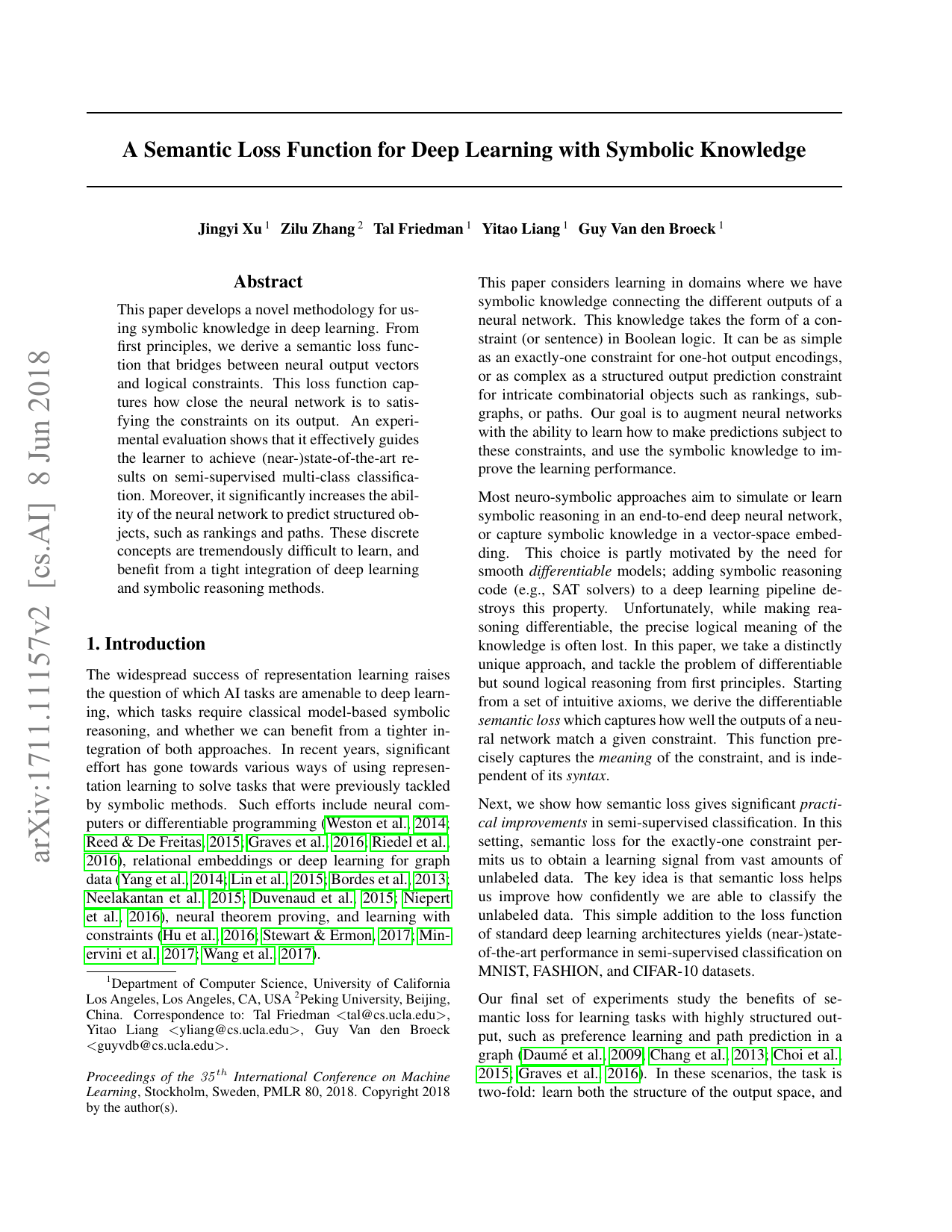
Figure 2: Why Unlabeled Data Can Matter
Comparison with Other Methods
Semantic Loss vs. LogicNet
Aspect
LogicNet
Semantic Loss
Rule interface
posterior projection
direct loss term
Intermediate object
teacher distribution $q^\star$
no intermediate teacher
Optimization route
project distribution, then distill
update parameters directly
Numerical object
soft truth / rule energy in a projected posterior
total probability mass of satisfying worlds
Semantic focus
posterior after rule correction
exact satisfying mass
LogicNet: modify the distribution first, then modify the parameters.Semantic Loss: modify the parameters directly through a logic-derived loss.Semantic Loss vs. DL2
Aspect
Semantic Loss
DL2
Logic object
set of satisfying assignments
declarative constraint formula
Numerical form
total satisfying probability mass
continuous surrogate violation or feasible-set objective
Semantic precision
high; retains exact logical meaning
depends on the surrogate design
Gradient geometry
globally coupled
more local, piecewise, and design-dependent
Main bottleneck
logic compilation and counting complexity
surrogate design and inner search
A Useful Three-Way Compression
Why the Method Can Be Effective
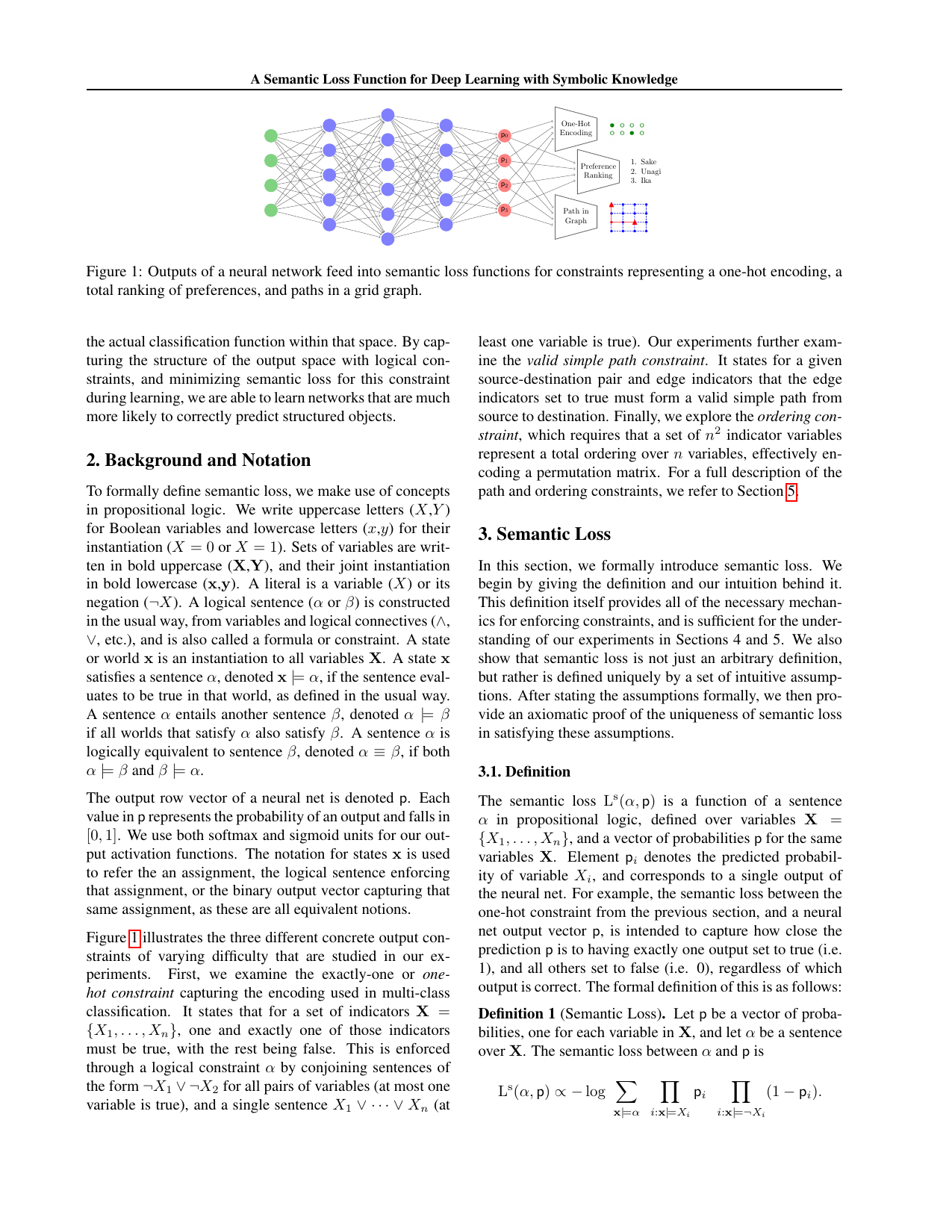
Semi-Supervised Classification
Structured Outputs
Limitations and Insights
Computation Can Dominate
exactly-one, the expression simplifies to
$$
\sum_{i=1}^m p_i\prod_{j\ne i}(1-p_j),
$$
which is cheap. For richer logical structures, the cost may become the central issue.Best Suited to Propositional Discrete Structures
Exact Semantics Does Not Guarantee Easy Optimization
Core Insight
Repository Alignment
logsumexp.logsigmoid and logsumexp is simply the numerically stable implementation of the same semantic definition.Minimal Reproduction Suggestions
exactly-one, because it is simultaneously:
sigmoid to obtain four independent Bernoulli probabilities;exactly-one Semantic Loss;
baseline vs. exactly_oneexactly_one vs. at_least_oneexactly_one vs. exactly_two_badCondensed Takeaway